What is Gradient Descent?
Gradient Descent is an iterative optimization algorithm used to adjust a model’s parameters in order to minimize its cost function. It’s a fundamental cornerstone of machine learning, and enables the “learning” part. It’s used in Neural Networks and Deep Learning models as well.
Our linear regression cost model only has 2 params, but we can use Gradient Descent on many various cost functions that have more than 2 parameters.
The cost function plotted below is NOT the squared error cost function for linear regression, thus there are multiple local minima (multiple minimum error rates)
When initiating Gradient Descent, you choose a random point to start. For example, during linear regression we usually start at the coordinates or . For the below example let’s start at the top of the crest where our happy little person is. Your goal is to find your way to one of the troughs, or local minima, as efficiently as possible.
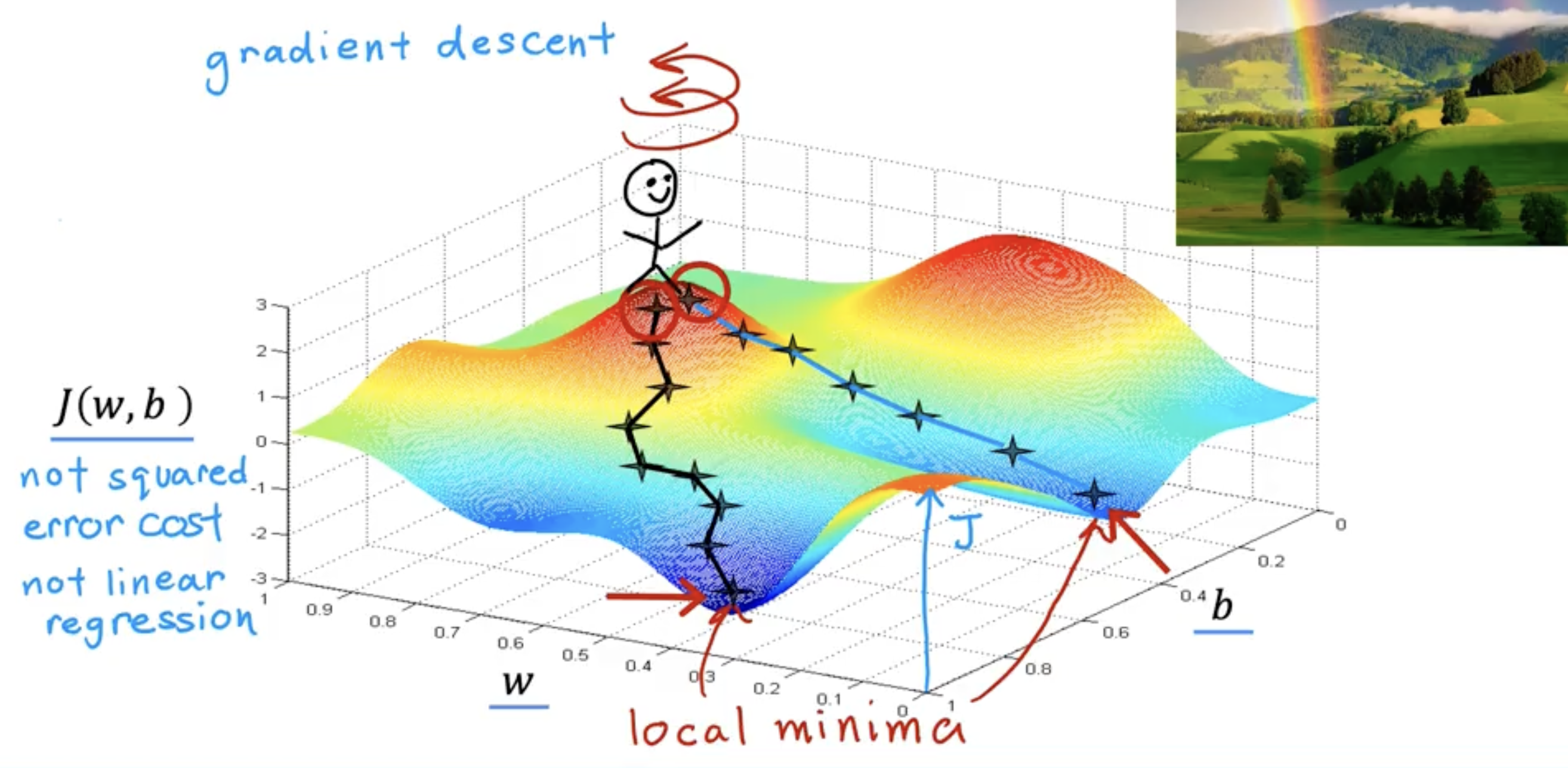
The Gradient descent algorithm essentially does a 360 turn at your current point and asks “if I were to take a tiny little baby step in one direction, and I want to go downhill as quickly as possible to one of these valleys. What direction do I choose to take that baby step?” That direction has the “steepest descent.”
We essentially repeat this process iteratively until we can no longer find a “steepest descent,” thus leaving us at our local minima/minimized error rate.
NOTE: you can see there are 2 paths that could lead you to two different local minima depending on where you start. Even though the origin point of the two paths are right next to each other, they arrive at different local minima.
Implementing Gradient Descent
So what is the Gradient Descent Algorithm?
- = The learning rate: A small positive number between 0 and 1. Controls how big of a step you take downhill. A large alpha means an aggressive gradient descent procedure
- = The derivative: Tells you which direction to take your baby step. Technically a partial derivative since we are only changing so many dimensions at a time while freezing the rest.
Intuition: The equal sign is the assignment operator. So you take the value and store it in w. So if the param a = a+1, then a=2. So then if you do a=a+1 again, a=3. With this in mind, we know we will have to update params w and b. Which means we need to write an assignment to update the param b:
In the graph of the surface plot, for the gradient descent algorithm, you need to repeat those two update steps until the algorithm converges. This means you reach the point at a local minimum where the parameters w and b no longer change much with each additional step that you take.
IMPORTANT: When implementing/calculating the gradient for multiple params, we need to update all the params simultaneously. This is because we do NOT want to update params during a single pass.
Think about it, if you need to update w and b in pass 1 you can’t update w and then calculate b afterwards using that updated w value in pass 1.. You need to update w, then wait for b to update with the old value of w, AND THEN continue to pass 2.
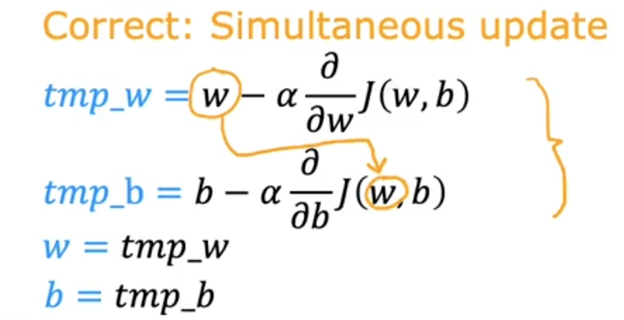
If we update w while calculating b, we would get the wrong next param value. This is why GPUs are so good for modern ML, because you can update so many params in one pass in parallel, then assign them all, THEN move on to step 2. This is for huge neural networks with billions of params.
but generally, simultaneous update doesn’t mean simultaneous computation. It means all gradients for a step must be calculated using the same current parameter values before those parameters are updated.
NOTE: gradient descent doesn’t know what a good model is. It only knows how to reduce the objective you give it
Gradient descent is an algorithm for finding values of parameters w and b that minimize the cost function J. What does this update statement do? (Assume is small.)
Answer: Updates the parameter by a small amount, in order to reduce the cost .
Gradient Descent Intuition
So far, we know the Gradient Descent Algo requires updating all params for our cost function J (w, b)
with the same learning rate until we reach convergence.
Let’s understand what the learning rate and derivative are doing, and why multiplying them repeatedly results in updates to w and b that make sense. To do this, let’s say our cost function only had 1 param… J (w).
This would mean our Gradient Descent Algo looks like this:
We are trying to minimize the cost by adjusting the parameter, w
TODO: Flesh this section of notes out
Shows the intuition that derivative here acts as a tangent to the cost function with a slope, and the slope will be positive/negative depending on which direction your gradient descent function has you moving along the cost function to find a local minima.
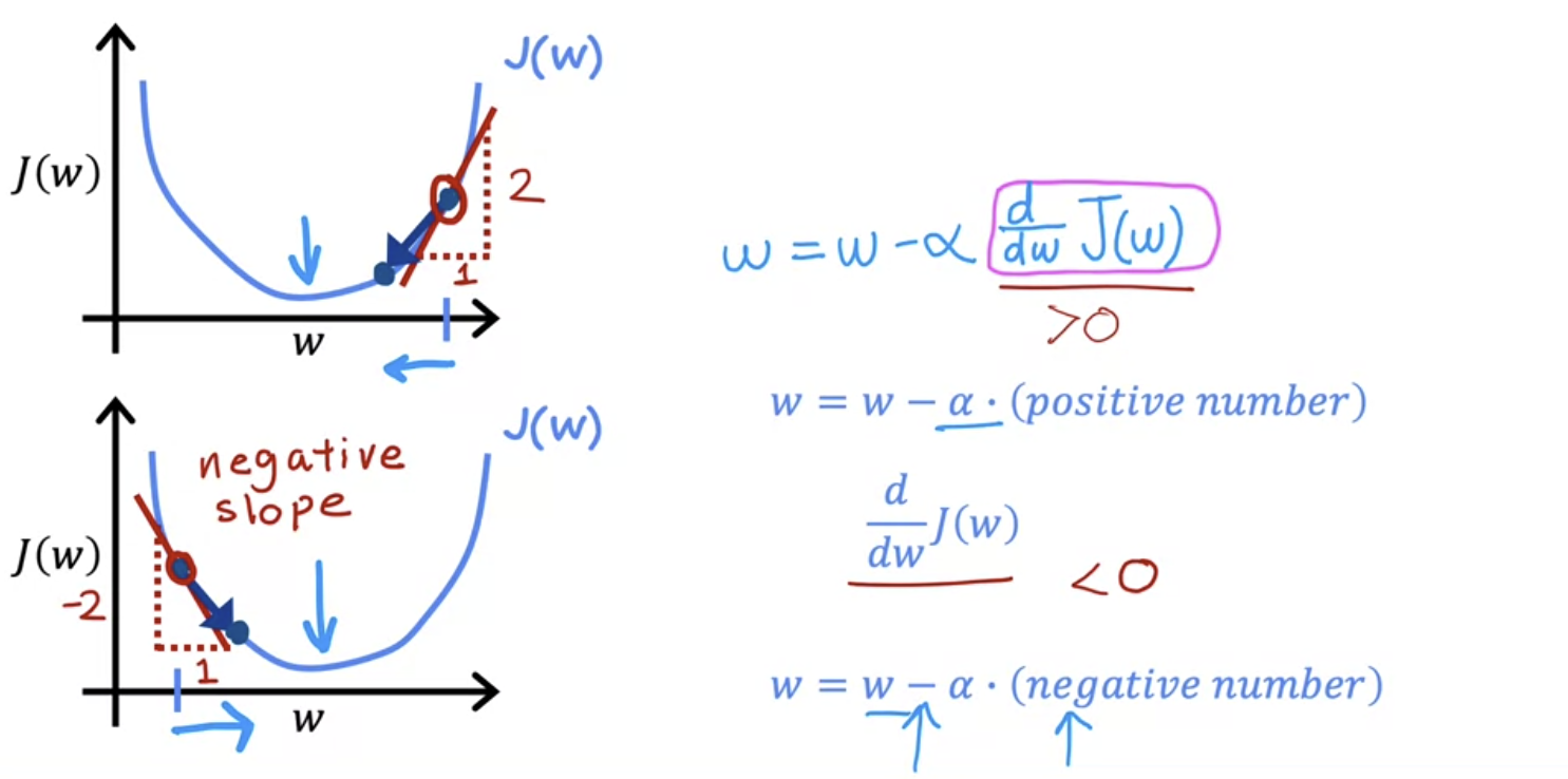
Based on the slide shown above, assuming the learning rate is a small positive number, when the derivative is a positive number what happens to w after one step?
Answer: decreases
The Learning Rate
The choice of the learning rate will have a huge affect on the efficiency of your gradient descent algorithm.
If is too small…
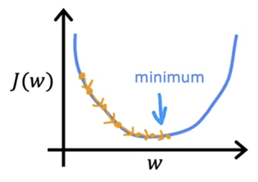
You’ll multiply your derivative term by a really small number, which means you’ll take a very small baby step down to the local minima. This means you’ll be decreasing the learning cost J, but very slowly. This is inefficient.
If is too large…
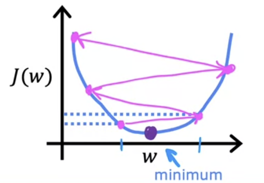
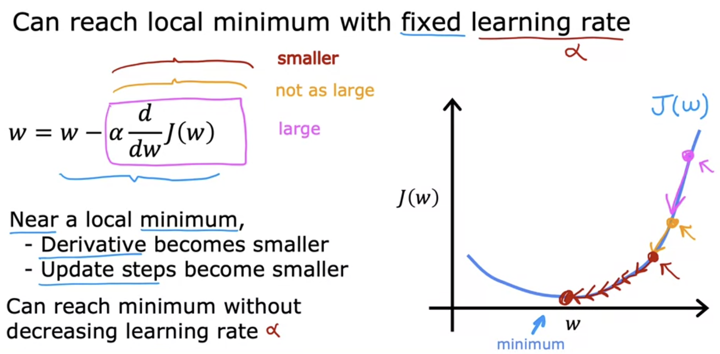
You’ll risk taking too large of a step closer to the minima, overstepping and making the cost for J(w) even worse. And once you take a step back, it’s possible you’ll keep stepping further away from the minima and failing to converge and potentially even diverging from the local minima.
TODO: Flesh this section of notes out
Shows that a constant learning rate works because as you keep updating your params with the gradient descent algorithm, the slope of the derivative will keep decreasing as it’s approaching the local minima, and will keep taking smaller steps. meaning it wont overshoot on your local minimum.